Kibble-Zurek quench in 2D transverse-field Ising model#

This example provides a quick overview of simulating the real-time Kibble-Zurek quench in 2D Ising model using YASTN library. We show an example of a system defined on a \(4{\times}4\) square lattice with open boundary conditions (OBC). The Hamiltonian reads

\[H(s) = f(s) \sum_{\langle i, j \rangle} J_{i,j} \sigma^x_i \sigma^x_j - g(s) \sum_i \sigma^z_i,\]

where \(\sigma^x\) and \(\sigma^z\) are standard Pauli matrices, and we assume random nearest-neighbor couplings \(J_{i,j} \in [-1, 1]\).

The amplitude of couplings is gradually turned on as \(f(s) = 1 + \sin(\pi (s - 0.5))\), and the transverse field is gradually turned off as \(g(s) = 1 - \sin(\pi (s - 0.5))\).

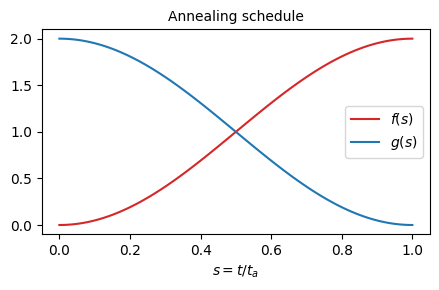
The system is initialized in the ground (product) state at \(s=0\), where the couplings \(f(0)=0\). The evolution ends upon reaching \(s=1\), where transverse field \(g(0)=0\). The quench rate is controlled by an annealing time \(t_a\) as \(s= t / t_a\). The system gets excited while passing the quantum critical point between paramagnetic and spin-glass phases in finite annealing time \(t_a\). This provides a minimal example of a class of problems considered in https://arxiv.org/abs/2403.00910

We compare the results obtained using MPS and PEPS routines. This example can be also run from tests/quickstart/test_KZ.py <https://github.com/yastn/yastn/blob/master/tests/quickstart/test_KZ.py>

Initialization of Model Parameters:

import math
import numpy as np
import matplotlib.pyplot as plt
from tqdm import tqdm  # progressbar
import yastn
import yastn.tn.mps as mps
import yastn.tn.fpeps as peps
from yastn.tn.fpeps.gates import gate_nn_Ising, gate_local_field
#
# Employ PEPS lattice geometry for sites and nearest-neighbor bonds
Lx, Ly = 4, 4  # lattice size
geometry = peps.SquareLattice(dims=(Lx, Ly), boundary='obc')
sites = geometry.sites()  # list of lattice sites
#
# Draw random couplings from uniform distribution in [-1, 1].
np.random.seed(seed=0)
Jij = {k: 2 * np.random.rand() - 1 for k in geometry.bonds()}
#
# Define quench protocol
fXX = lambda s : 1 + math.sin((s - 0.5) * math.pi)
fZ  = lambda s : 1 - math.sin((s - 0.5) * math.pi)
ta = 2.0  # annealing time
dt = 0.04  # intended time step; make it smaller to decrease errors
steps = round(ta / dt)  # enforce integer number of Trotter steps
dt = ta / steps
#
# Load operators. Problem has Z2 symmetry, which we impose.
ops = yastn.operators.Spin12(sym='Z2')

PEPS simulations; time evolution:

def gates_Ising(Jij, fXX, fZ, s, dt, sites, ops):
    """ Trotter gates at time s. """
    nn, local = [], []
    # time-step is 1j * dt / 2, as trotterized evolution is
    # completed by its adjoint for 2nd order time-evolution method.
    dt2 = 1j * dt / 2
    for bond, J in Jij.items():
        gt = gate_nn_Ising(J * fXX(s), dt2, ops.I(), ops.x(), bond)
        nn.append(gt)
    for site in sites:
        gt = gate_local_field(fZ(s), dt2, ops.I(), ops.z(), site)
        local.append(gt)
    return peps.Gates(nn=nn, local=local)
#
# Initialize system in the product ground state at s=0.
psi = peps.product_peps(geometry=geometry, vectors=ops.vec_z(val=1))
#
# simulation parameters
D = 6  # PEPS bond dimension
opts_svd_ntu = {"D_total": D}
#
env = peps.EnvNTU(psi, which='NN+')
# The environment used to calculate bond metric tensor.
# This is a setup for NTU NN+ environment as described in
# the appendix of https://arxiv.org/abs/2403.00910
#
infoss = []  # for diagnostics information
#
# execute time evolution
t = 0
for _ in tqdm(range(steps)):
    t += dt / 2
    gates = gates_Ising(Jij, fXX, fZ, t / ta, dt, sites, ops)
    infos = peps.evolution_step_(env, gates, opts_svd=opts_svd_ntu)
    # The state psi is contained in env
    # evolution_step_ updates psi in place.
    infoss.append(infos)
    t += dt / 2

Delta = peps.accumulated_truncation_error(infoss, statistics='mean')
print(f"Accumulated mean truncation error: {Delta:0.5f}")

PEPS simulations; final correlations:

# We employ boundary MPS to contract the network
opts_svd_env = {'D_total': 4 * D}
opts_var_env = {"max_sweeps": 8,
                "overlap_tol": 1e-5,
                "Schmidt_tol": 1e-5}
#
# setting-up environment
env_mps = peps.EnvBoundaryMPS(psi,
                              opts_svd=opts_svd_env,
                              opts_var=opts_var_env, setup='lr')
#
# Calculating 1-site <Z_i> for all sites
Ez_peps = env_mps.measure_1site(ops.z())
#
# Calculating 2-site <X_i X_j> for all pairs i <= j
Exx_peps = env_mps.measure_2site(ops.x(), ops.x(),
                                 opts_svd=opts_svd_env,
                                 opts_var=opts_var_env)

MPS simulations:

# Map between sites and linear MPS ordering.
s2i = {s: i for i, s in enumerate(sites)}
#
# Map for bonds, sorting pairs of MPS indices for convinience
b2i = lambda s1, s2: tuple(sorted([s2i[s1], s2i[s2]]))
#
# define Hamiltonian MPO
HI = mps.product_mpo(ops.I(), N=Lx*Ly)  # identity MPO
#
termsXX = [mps.Hterm(amplitude=J,
                     positions=[s2i[s1], s2i[s2]],
                     operators=[ops.x(), ops.x()]) \
            for (s1, s2), J in Jij.items()]
HXX = mps.generate_mpo(HI, termsXX)
#
termsZ = [mps.Hterm(-1, i, ops.z()) for i in range(Lx * Ly)]
HZ = mps.generate_mpo(HI, termsZ)
#
# MPO contributions in H(t) will be added up.
H = lambda t: [HXX * fXX(t / ta), HZ * fZ(t / ta)]
#
# Initial state. TDVP is unstable starting in a product state
# There are many strategies to mitigate it.
# Here, a simple strategy to start with a product state obtained
# via DMRG with artificially enlarged bond dimension is sufficient.
psi = mps.random_mps(HI, D_total=16)  # initialize with D=16
mps.dmrg_(psi, H(0), method='1site', max_sweeps=8, Schmidt_tol=1e-8)
#
# time-evolution generator and its parameters
opts_expmv = {'hermitian': True, 'tol': 1e-12}
opts_svd = {'tol': 1e-6, 'D_total': 64}  # max MPS bond dimension
evol = mps.tdvp_(psi, H, times=(0, ta),
                method='12site', dt=dt, order='2nd',
                opts_svd=opts_svd, opts_expmv=opts_expmv,
                progressbar=True)
#
# run evolution
# evol is a generator with one (final) snapshot to reach
next(evol)  # execute time evolution
#
# calculate expectation values
Ez_mps = mps.measure_1site(psi, ops.z(), psi)
Exx_mps = mps.measure_2site(psi, ops.x(), ops.x(), psi, bonds="<=")

Compare results of PEPS and MPS:

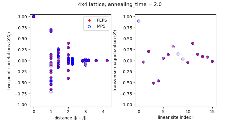
Z_peps = np.array([Ez_peps[st].real for st in sites])
Z_mps = np.array([Ez_mps[s2i[st]].real for st in sites])
error_Z = np.linalg.norm(Z_peps - Z_mps) / np.linalg.norm(Z_mps)
print(f"Relative difference of PEPS vs MPS in Z magnetization: {error_Z:0.5f}")

# Euclidian distance on a square lattice
dist = lambda s1, s2: np.linalg.norm([s1[0]-s2[0], s1[1]-s2[1]])
rs = np.array([dist(s1, s2) for (s1, s2) in Exx_peps])
#
XX_peps = np.array([*Exx_peps.values()]).real
XX_mps = np.array([Exx_mps[b2i(*bond)] for bond in Exx_peps.keys()]).real
error_XX = np.linalg.norm(XX_peps - XX_mps) / np.linalg.norm(XX_mps)
print(f"Relative difference of PEPS vs MPS in XX correlations: {error_XX:0.5f}")

Visualize:

fig, ax = plt.subplots(1, 2)
fig.set_size_inches(8, 4)
plt.subplots_adjust(hspace=0.3, wspace=0.3)
ax[0].scatter(rs, XX_peps, label='PEPS',
            marker='+', color='r')
ax[0].scatter(rs, XX_mps, label='MPS',
            marker='o', color='b', facecolors='none')
ax[0].set_ylim([-1.05, 1.05])
ax[0].set_xlabel(r"distance $||i - j||$")
ax[0].set_ylabel(r"two-point correlations $\langle X_i X_j \rangle$")
ax[0].legend()
ax[1].scatter(np.arange(len(Z_peps)), Z_peps, label='PEPS',
                marker='+', color='r')
ax[1].scatter(np.arange(len(Z_mps)), Z_mps, label='MPS',
                marker='o', color='b', facecolors='none')
ax[1].set_xlabel(r"linear site index i")
ax[1].set_ylabel(r"transverse magnetization $\langle Z_i \rangle$")
ax[1].set_ylim([-1.05, 1.05])
fig.suptitle(f"{Lx}x{Ly} lattice; annealing_time = {ta:0.1f}")
fig.show()

Kibble-Zurek quench in 2D transverse-field Ising model#

This Page